Posts

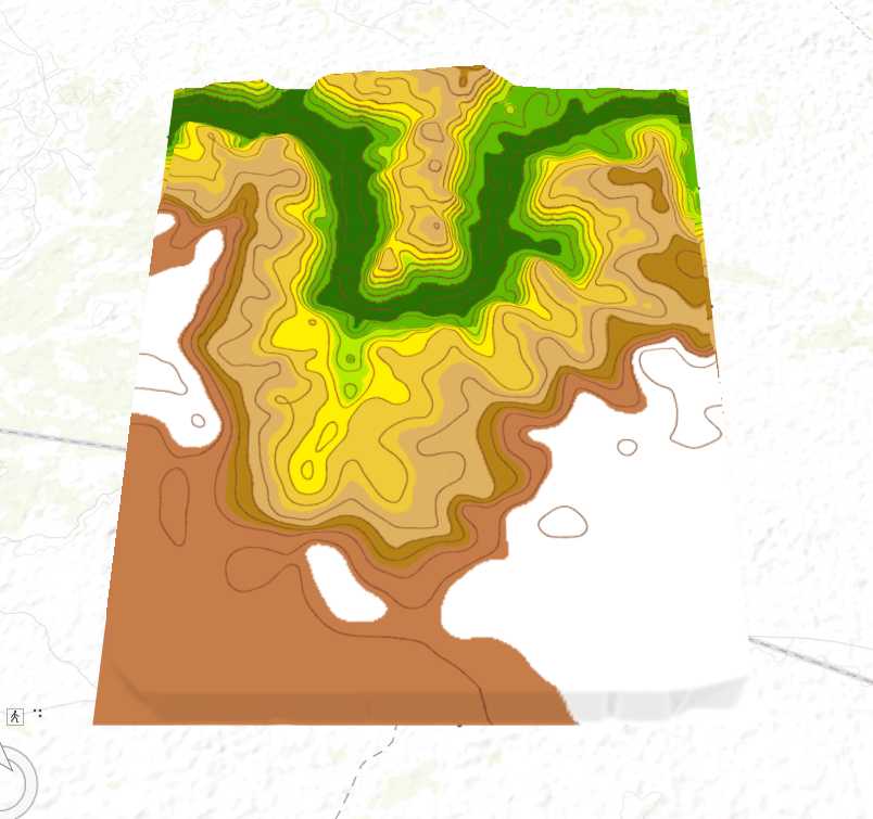
GIS5935 M2.1 Surfaces - TINs and DEMs
Image
In my exploration of elevation data models, I examined both Triangulated Irregular Networks (TINs) and Digital Elevation Models (DEMs) to understand their unique properties and applications. TINs are formed by connecting data points into triangles, providing highly detailed but angular representations of terrain. On the other hand, DEMs are grid-based and create smoother surface representations through interpolation techniques. I compared these models by analyzing contour lines generated from both TIN and DEM data. One key difference I found is that DEM contours are much smoother, especially in flatter areas with less elevation variation, while TIN contours are more angular, especially in areas of steeper terrain due to the triangular structure. The smoother DEM is more suitable for continuous surface representation, while the TIN excels in areas requiring more detailed elevation information. A comparison between DEM and TIN contours can be seen below: DEM TIN This exploration highligh...

GIS5935 M1.2 Data Quality Assessment

Image
 Accuracy Assessment of Road Network Completeness Goal of the Accuracy Assessment This accuracy assessment aims to compare the completeness of two road network datasets: Street_Centerlines and TIGER_Roads shapefiles for Jackson County, Oregon. The objective of evaluating the total length of roads within a uniform 5km x 5km grid is to determine which dataset provides more comprehensive coverage for the area. This analysis allows for identifying areas where one dataset may be more detailed than the other, contributing to a better understanding of road network quality in the region. Analysis Methodology The analysis methodology involved multiple steps to compare the two road networks. First, the road datasets— Street_Centerlines.shp and TIGER_Roads.shp —were clipped to the boundaries of a 5km x 5km grid that spans Jackson County. The Clip  tool ensured that the roads outside the grid cells were removed. The next step used the Intersect tool to divide road segments at the grid b...

GIS5935 M1.2 Lab Data Standards

Image
  Assessing Positional Accuracy of Road Networks: A Case Study In this project, I conducted an accuracy assessment of road networks using data from the city of Albuquerque and StreetMap USA. The goal was to determine the positional accuracy of the two datasets, following the methodology outlined by the National Standard for Spatial Data Accuracy (NSSDA).  Below is a screenshot of the test point locations for the data from the city of Albuquerque: Steps Taken to Complete the Accuracy Assessment: Data Exploration : I began by exploring both datasets, comparing road centerlines from the City of Albuquerque and StreetMap USA against orthophotos of the area to check for differences. Selection of Test Points : Using NSSDA guidelines, I selected 20 well-defined points, such as road intersections, that were visible in both datasets and the reference orthophotos. Independent Dataset : The orthophotos were treated as the independent reference data due to their high level of accuracy. Co...

GIS5935 M1.1 Lab

Image
Exploring GPS Data Accuracy and Precision: A Brief Analysis Numerical Results for Horizontal Accuracy and Precision Horizontal Accuracy: 3.24 meters Horizontal Precision (68%): 4.47 meters Understanding Horizontal Accuracy and Precision Horizontal Accuracy: This is the measure of how close the average of the collected waypoints is to the true location (not shown in the map). In this case, the average waypoint is 3.24 meters away from the true reference point, indicating reasonably accurate measurements. Horizontal Precision: Precision refers to the spread or variability of the GPS points around the average. Here, a precision of 4.47 meters suggests that the individual measurements are spread out, meaning that while the average position is accurate, the data points themselves are not consistent. This difference between accuracy and precision highlights the GPS unit's performance: it provides a generally accurate estimate of the location, but has low precision with variability in ...

M6 - Least Cost

Image
  Habitat Suitability and Corridor Analysis Introduction In this post, I’ll share the process and results of a habitat suitability and corridor analysis aimed at identifying the most suitable areas for conservation and the optimal paths between protected regions. This analysis involved creating a habitat suitability model based on key environmental factors, followed by a corridor analysis to determine the best routes for wildlife movement between two National Forests. Analysis Steps The first step in the analysis was to create a habitat suitability model using three criteria: land cover, elevation, and proximity to roads. Each criterion was reclassified on a scale of 1 to 10 to reflect its relative suitability for wildlife habitat. I combined these reclassified layers using the Weighted Overlay tool, with land cover given a weight of 60%, elevation 20%, and distance to roads 20%. This produced a suitability raster highlighting the most appropriate areas for conservation. Next, I in...

M6 - Suitability Analysis

Image
  Introduction In this blog post, I present the outcomes of a development suitability analysis, focusing on a comparison between two distinct weighting scenarios. The objective was to identify the most favorable areas for development by considering five essential criteria: land cover, soils, slopes, proximity to streams, and proximity to roads. Analysis Steps The analysis started by reclassifying each of the five criteria into a suitability scale from 1 (least suitable) to 5 (most suitable). Initially, all criteria were assigned equal weights of 20%, ensuring an unbiased approach in combining the factors for the suitability model. Then, an alternative scenario was explored, where slopes were given a greater emphasis with a 40% weight, while the remaining criteria—land cover and soils—were weighted at 20% each, and proximity to streams and roads at 10% each. These criteria were integrated using the Weighted Overlay tool, resulting in two final suitability maps. The first map display...

M4 - Coastal Flooding

Image
  Harnessing GIS for Coastal Flooding Analysis: A Deep Dive into Technology and Techniques Introduction Coastal regions, increasingly vulnerable in the face of climate change, are finding Geographic Information Systems (GIS) to be essential tools for managing the devastating impacts of flooding and erosion. This blog post explores the utilization of GIS technologies in assessing coastal flood risks, focusing on erosion analysis and storm surge predictions. Understanding Erosion Through GIS Analyzing coastal erosion involves multiple sophisticated steps that leverage advanced mapping and data collection via GIS. In places like Mantoloking, New Jersey, detailed assessments can capture significant landform changes before and after events such as hurricanes, thanks to high-resolution LiDAR data. This kind of detailed analysis is crucial for effective coastal management. Analyzing Storm Surge Impact In hurricane-prone areas, the potential damage from storm surges can be modeled extensiv...